Getting Started

Setting up R packages

packages = c('sf', 'tmap', 'tidyverse', 'lubridate', 'clock',
             'sftime', 'rmarkdown')

for(p in packages){
  if(!require(p, character.only = T)){
    install.packages(p)
  }
  library(p, character.only = T)
}

Importing Data

schools <- read_sf("data/wkt/Schools.csv", 
                   options = "GEOM_POSSIBLE_NAMES=location")

apartments <- read_sf("data/wkt/Apartments.csv", 
                   options = "GEOM_POSSIBLE_NAMES=location")

buildings <- read_sf("data/wkt/Buildings.csv", 
                   options = "GEOM_POSSIBLE_NAMES=location")

employers <- read_sf("data/wkt/Employers.csv", 
                   options = "GEOM_POSSIBLE_NAMES=location")

pubs <- read_sf("data/wkt/Pubs.csv", 
                   options = "GEOM_POSSIBLE_NAMES=location")

restaurants <- read_sf("data/wkt/Restaurants.csv", 
                   options = "GEOM_POSSIBLE_NAMES=location")

logs <- read_sf("data/wkt/ParticipantStatusLogs1.csv", 
                options = "GEOM_POSSIBLE_NAMES=currentLocation")

Checking the data

print(schools)

Simple feature collection with 4 features and 4 fields
Geometry type: POINT
Dimension:     XY
Bounding box:  xmin: -4701.463 ymin: 1607.984 xmax: -376.7505 ymax: 6556.032
CRS:           NA
# A tibble: 4 × 5
  schoolId monthlyCost maxEnrollment             location
  <chr>    <chr>       <chr>                      <POINT>
1 0        12.81244502 242           (-376.7505 1607.984)
2 450      91.14351385 418           (-2597.448 3194.155)
3 900      38.00537955 394           (-2539.158 6556.032)
4 1350     73.19785215 384           (-4701.463 5141.763)
# … with 1 more variable: buildingId <chr>

print(buildings)

Simple feature collection with 1042 features and 4 fields
Geometry type: POLYGON
Dimension:     XY
Bounding box:  xmin: -4762.191 ymin: -30.08359 xmax: 2650 ymax: 7850.037
CRS:           NA
# A tibble: 1,042 × 5
   buildingId                       location buildingType maxOccupancy
   <chr>                           <POLYGON> <chr>        <chr>       
 1 1          ((350.0639 4595.666, 390.0633… Commercial   ""          
 2 2          ((-1926.973 2725.611, -1948.1… Residental   "12"        
 3 3          ((685.6846 1552.131, 645.9985… Commercial   ""          
 4 4          ((-976.7845 4542.382, -1053.2… Commercial   ""          
 5 5          ((1259.306 3572.727, 1299.255… Residental   "2"         
 6 6          ((478.8969 1082.484, 473.6596… Commercial   ""          
 7 7          ((-1920.823 615.7447, -1960.8… Residental   ""          
 8 8          ((-3302.657 5394.354, -3301.5… Commercial   ""          
 9 9          ((-600.5789 4429.228, -495.95… Commercial   ""          
10 10         ((-68.75908 5379.924, -28.782… Residental   "5"         
# … with 1,032 more rows, and 1 more variable: units <chr>

Plotting the building footprint map

tmap_mode(“view”): is for switch-on and tmap_mode(“plot”) is for switch-off interactivity tm_shape: define the geometric data border.lwd: width

tmap_mode("view")
tm_shape(buildings)+
tm_polygons(col = "grey60",
           size = 1,
           border.col = "black",
           border.lwd = 1)

tmap_mode("plot")

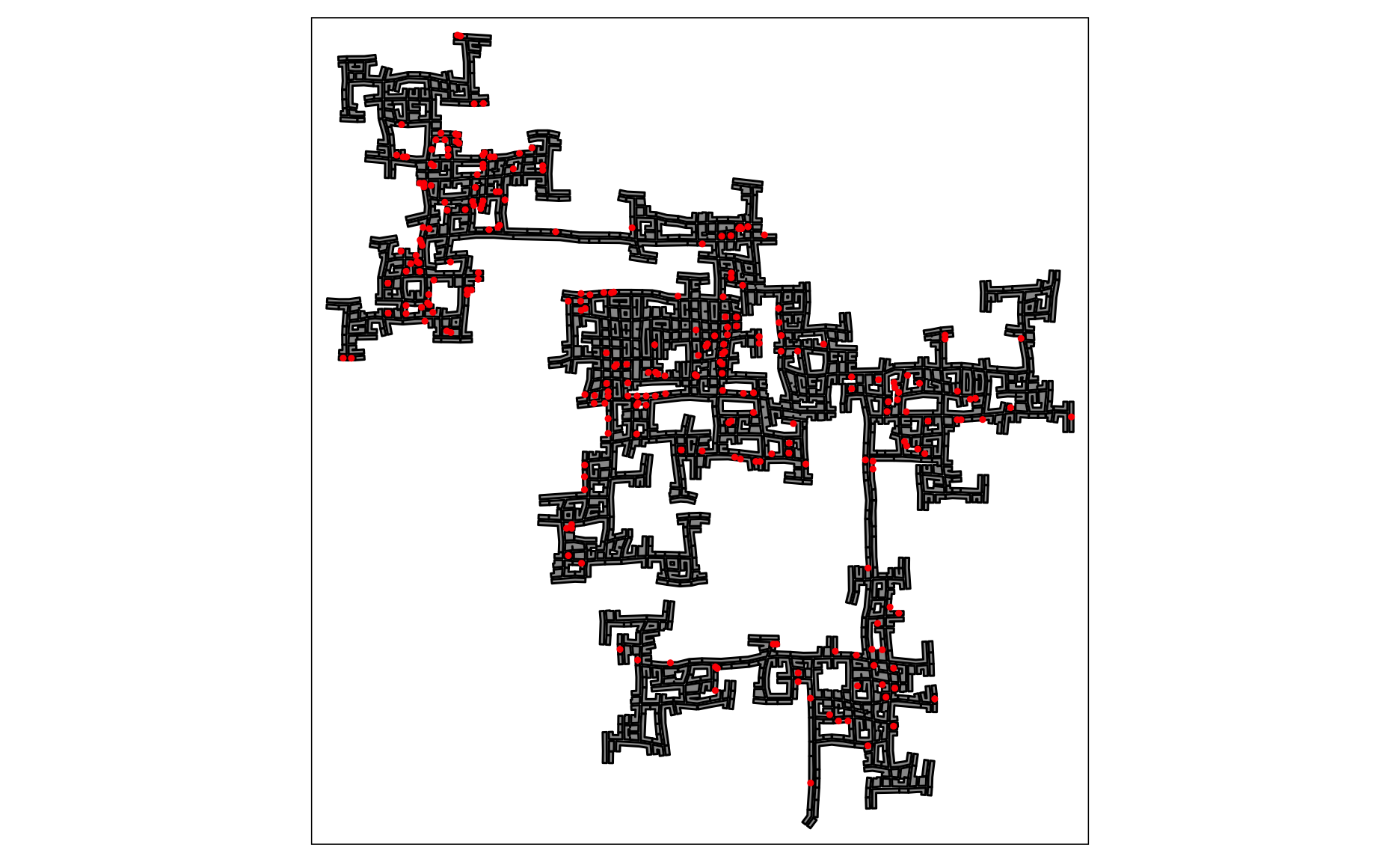
Plotting a composite map

Remember to plot the area first before plotting the line and points, since the tm_ploygons would cover the point.

tmap_mode("plot")
tm_shape(buildings)+
tm_polygons(col = "grey60",
           size = 1,
           border.col = "black",
           border.lwd = 1) +
tm_shape(employers) +
  tm_dots(col = "red")

Converting timestamp field in movement data

logs_selected <- logs %>%
  mutate(Timestamp = date_time_parse(timestamp,
                                     zone = "",
                                     format = "%Y-%m-%dT%H:%M:%S")) %>%
  mutate(day = get_day(Timestamp)) %>%
  filter(currentMode == "Transport")

Plotting Hexagon Binning Map

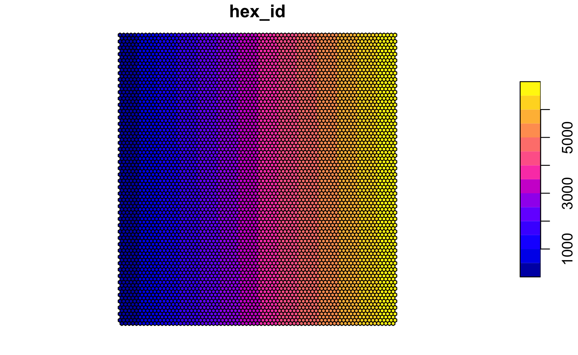
Computing the haxegons

hex <- st_make_grid(buildings, 
                    cellsize=100, 
                    square=FALSE) %>%
  st_sf() %>%
  rowid_to_column('hex_id')
plot(hex)

Performing point in polygon overlay

points_in_hex <- st_join(logs_selected, 
                         hex, 
                         join=st_within)
#plot(points_in_hex, pch='.')

Performing point in polygon count

points_in_hex <- st_join(logs_selected, 
                        hex, 
                        join=st_within) %>%
  st_set_geometry(NULL) %>%
  count(name='pointCount', hex_id)
head(points_in_hex)

# A tibble: 6 × 2
  hex_id pointCount
   <int>      <int>
1    169         35
2    212         56
3    225         21
4    226         94
5    227         22
6    228         45

Performing relational join

hex_combined <- hex %>%
  left_join(points_in_hex, 
            by = 'hex_id') %>%
  replace(is.na(.), 0)

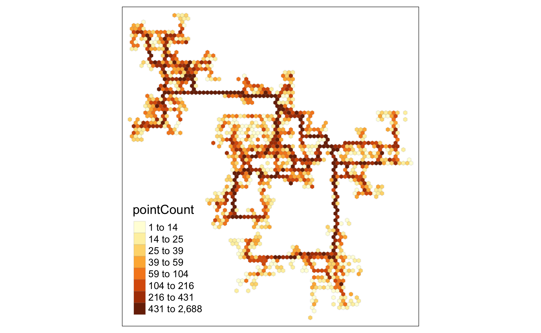
Plotting the hexagon binning mapp

tm_shape(hex_combined %>%
           filter(pointCount > 0))+
  tm_fill("pointCount",
          n = 8,
          style = "quantile") +
  tm_borders(alpha = 0.1)

Plotting Movement Path

Creating movement path from event points

logs_path <- logs_selected %>%
  group_by(participantId, day) %>%
  summarize(m = mean(Timestamp), 
            do_union=FALSE) %>%
  st_cast("LINESTRING")

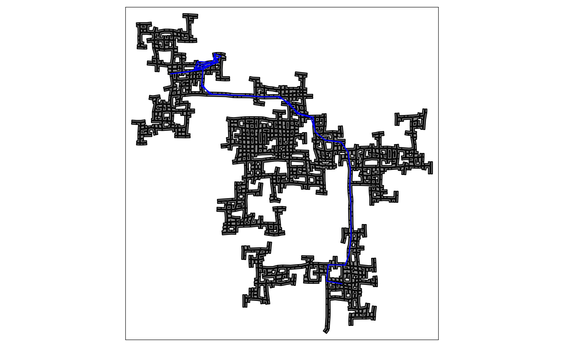
Plotting the Movement Paths

logs_path_selected <- logs_path %>%
  filter(participantId==0)
tmap_mode("plot")
tm_shape(buildings) +
tm_polygons(col = "grey60",
            size = 1,
            border.col = "black",
            border.lwd = 1) +
  tm_shape(logs_path_selected) +
  tm_lines(col = "blue")

tmap_mode("plot")

In-class Exercise 6